September 30, 2022, by Digital Research
Using Julia on the HPC
In this blog, we explore the speed and efficiency of using the programming language Julia on the University’s high-performance computer.
This blog has been guest-authored by Jamie Mair, a PhD researcher in the School of Physics and Astronomy.
The repository for the code given below, which was presented at this year’s annual UoN HPC conference, can be found here.
For more information on the University’s high-performance computer, please see here.
What is Julia?
Julia is a modern, general purpose, programming language. It was designed for high-performance scientific programming. According to a blog post written by the creators, Julia was borne out of the desire for a programming language which is as fast as C, yet easy to use like Python, MATLAB and R. Personally, I use Julia because it is incredibly easy to prototype new code for my research, while being flexible enough to execute my code across my home machine, my GPU or an entire cluster. And all of this with minimum effort on my part!
In this blog, I discuss what’s possible in Julia for very little investment. You will see how to write reusable code and take advantage of every level of parallelism, from the hardware parallelism of SIMD, to executing native Julia code on the GPU and scaling it across a cluster. The ease of use and flexibility of this parallelism is unmatched and provides a very low bar to entry.
Julia is fast
Julia has many advantages when compared to other languages. However, the main claim that will interest our HPC community is speed. Julia claims to be as fast as C, so let’s put that to the test.
I will use the example of simulating a Monte-Carlo process, specifically a random walk. This process is simple, but the basics are used in a wide variety of fields and are common in HPC workloads.
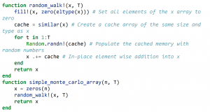
The code for running a random walk is:
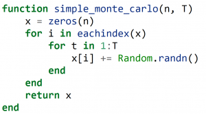
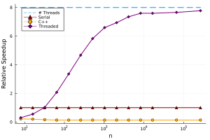
This function performs n random walks, all of length T. We can write some code in C++ that is roughly equivalent, to see empirical differences in performance.
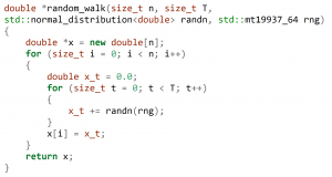
This implementation in C++ is not optimal at all (I am no C++ programmer), but is indicative of what a typical PhD student might write for simulations. We find that the Julia version is between 4 and 7 times faster (depending on the size of n).
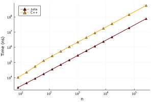
While Julia has the advantage here, I don’t think that Julia is inherently faster than C/C++. A better C/C++ developer could make the C/C++ code perform similar to the Julia code. The main point I want to make is that you can achieve C/C++ levels of performance for minimal effort, while keeping your code simple and trusting Julia’s “Just in Time” compiler (the standard LLVM compiler) to produce fast machine code. Not all code will run quickly, but there are performance tips that will let you achieve these C-like speeds.
Multi-threading in Julia
Almost every modern CPU has multiple cores, thus providing additional compute power. Julia provides lightweight multi-threading support natively. The language provides many ways of parallelising your code, but here we’ll just use a macro to make this process easy. A macro is code that writes other code. For executing a loop in parallel, we just add an @threads macro from the standard Threads library:
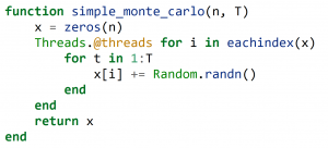
This is essentially the same source code as above, with just a simple change in front of the for-loop. We can add this to the performance graph:
We can see that this is pretty good performance out of the box. Unfortunately, we can see that threading doesn’t reach the theoretical maximum speedup, though there are techniques to remedy this.
Moving to the GPU
The modern GPU excels at array-based operations at scale, such as standard BLAS operations (matrix multiplications, etc.), which make up the backbone of a lot of numerical and scientific computing. Writing code for a GPU is notoriously difficult (custom kernels in C present a high barrier to entry for beginners).
The good news is that Julia has a successful package, called CUDA.jl, which allows you to write native Julia code that will compile directly to GPU code. Let’s take it for a spin!
Up to now, we have focused on using the standard Julia libraries, but there is a rich ecosystem of packages available. Adding a package is as simple as running the following code:
![]()
This uses Julia’s built-in package manager to download the CUDA.jl package. What makes this process painless is that when you use CUDA for the first time, it will download the CUDA libraries you need to get things working instead of having to install CUDA manually (as you need to do in Python libraries like Tensorflow and PyTorch).
GPUs are very different devices to CPUs and have a slightly different programming model. The main difference is that scalar indexing of an array has really poor performance on a GPU, and so the CUDA.jl package errors when you try to do this. Instead, we can use Julia’s excellent “broadcasting” notation, which allows us to write concise “vectorised” code. This notation also allows us to write non-allocating code, which means that we can reuse memory. This can make a huge performance difference. Here’s the same random walk code, rewritten to use array-based notation and avoiding allocating memory:
Please note that the use of the ! at the end of the function name is just notation that tells us that the function mutates the input arguments.
This code runs fine on the CPU with arrays, and is very similar to how someone would write this in MATLAB or numpy (in Python). We can benchmark this function and add it to the graph:
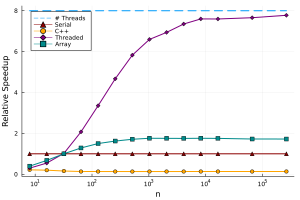
Notice that this has slightly better performance than the serial implementation, as it can make use of hardware SIMD instructions. What is really powerful about this approach is that we can directly re-use this code to run the code on the GPU:
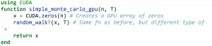
There are no changes to our code!
The only thing we changed was the type of our array. Since Julia has a Just-in-Time compiler, which specialises on the type of the input arguments, it knows to perform all of the array-based operations on x on the GPU. We can see the performance below:
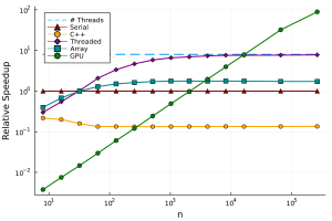
Here we can see that it is only really worth using the GPU for many elements in our array. If we require millions of calculations, the GPU can be around 100x faster than the CPU! We were able to get this huge increase in performance by only changing the input type to our function, and were able to reuse our original code.
Here, we have really only scratched the surface of GPU programming, as you can always move onto writing your own kernels from scratch. For a more detailed review, check out the CUDA.jl documentation.
Scaling up to cluster
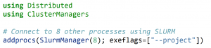
This wouldn’t be an HPC blog without talking about using a cluster. While it is certainly possible to use a single node with multi-threading, Julia also has native support for multiprocessing to scale across multiple nodes. Julia has native support for multiprocessing (with the Distributed.jl standard library that comes with Julia), and support for schedulers like SLURM with ClusterManagers.jl.
In order to connect all of the nodes, all we need to do is run the following code:
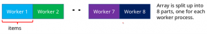
We could use the parallel primitives as described in the Distributed.jl documentation. But let’s reuse some of our previous code and take the array based programming model. There is a package called DistributedArrays.jl that gives us the DArray type. As the name suggests, this distributes the memory of an array in blocks to each process:
We would hope that we could copy the method of implementing the GPU extension:
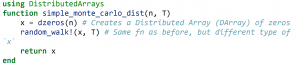
Unfortunately, the above code does not work on its own, but needs to implement the Random.randn! function for the DArray type. But since our function is easily mapped to each block in the DArray, we can just write a specific implementation of our random_walk! for this type, which we can do with a little help from the DistributedArrays.jl documentation:
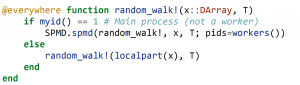
We have to use the @everywhere macro to load the function on each of the workers. Usually, you can put all the code that each worker needs in a separate file and just call @everywhere once.
This code just tells Julia how to call our original random_walk! function on each block of the array, reusing our code from before. The performance (for 8 workers) is added to our graph:
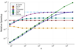
Multiprocessing always has a much higher overhead than multi-threading, but we can scale to potentially millions of processes, and use memory and resources from hundreds of different computers.
What’s next?
Hopefully, in this blog, I have shown you the potential of using Julia to enable a range of parallelism, and convince you that there is a low barrier to entry to get started! All of the code in this blog post can be found in the blog folder in this GitHub repository.
If you want to learn more about Julia, you can visit the website and if you want to learn the language, start with the Julia manual.
In this blog, I haven’t gone through many of the other reasons that people use Julia, such as multiple dispatch or state-of-the-art support for differential equations and scientific machine learning. If there are packages that you need and are only available in Python, there is also a package called PyCall.jl which will let you let you run and write Python code directly from Julia, giving you access to the entire Python ecosystem.
Finally, if you want to ask questions, there is a very active community on the Julia discourse.
For information and getting connected to the University of Nottingham HPC, please see here.
Happy programming!
Sorry, comments are closed!