June 3, 2021, by Rupert Knight

Using visual models to solve problems and explore relationships in Mathematics lessons – Part 2 (putting the theory into Practice)

This is the second of a two-part blog series by Marc North focused on using representations in Mathematics lessons to both solve problems and explore mathematical relationships. Part 1, available here, unpicked some of the key theoretical ideas around the use of representations and models. This Part 2 illustrates how these theoretical ideas can be applied practically.

A quick recap of the theory
The Teaching for Mastery approach has ushered in a dedicated focus on the use of different representations in Mathematics lessons. The Concrete-Pictorial-Abstract (CPA) heuristic frames much of this work and foregrounds sequences of learning that involve a combination of physical experiences and picture representations to support access to abstract mathematical concepts. Although the origins of this approach stem from Jerome Bruner’s work on enactive-iconic-symbolic representation modes, there are important differences with this early work that raise the potential for challenges with how the CPA is currently operationalised by some teachers. For example, some teachers see the CPA approach as hierarchical, with the ‘abstract’ dimension the ultimate goal. This leads to problematic practices such as using the CPA approach as a framework for differentiation, with lower-attainers encouraged to engage primarily with concrete and picture representations and higher attainers with abstract representations. Several of these sorts of challenges to the CPA were explored in more detail in Part 1.

While the CPA framework helps us to think about the different formats for representations or models, the Realistic Mathematics Education (RME) framework gives us a lens to discern different purposes or functions of models. There are three key features of RME that are helpful for this discussion – contexts, models, and the ‘progressive formalisation’ principle. By contextualizing mathematical contents in ‘realistic’ contexts (contexts that students can imagine and relate to), students are provided with an anchor in which to ground understanding of abstract contents. From here, models of a problem can be developed to represent and solve the problem. These models bear a close connection to the problem situation at hand – for example, using a picture of a pizza to represent a fraction of a whole. These models can then be developed further and generalized into models for representing, describing, and investigating mathematical structures and relationships over a range of problem situations and even content topics. These ‘Models for’ are powerful precisely because they allow us to investigate mathematical relationships and explore different ways of working. From a RME perspective, when using representations it is essential to choose models and representations that can easily be developed from models of a specific local situation to models for describing more general and abstract relationships. This progressive formalisation of models helps students navigate a learning trajectory to abstract concepts and equips them with a small number of models that have applicability over a range of problem and content types.

In an attempt to move beyond thinking only about different formats of representations (C or P or A), we have been applying these ideas about the different purposes of models in our PGCE sessions. This has helped us to explore how models and representations can be used not only to represent and solve problems (‘models of’), but also to investigate mathematical relationships and to compare and contrast different ways of working (‘models for’). The discussion below provides a practical example of this.

Using carefully chosen models to investigate mathematical relationships – practical illustration
Consider the following problem (and note that the problem is contextualised in a ‘realistic’ context):

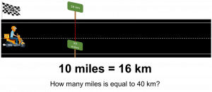
Figure 1: A conversion rate problem

There are a number of numerical methods for solving this problem – some are shown below.

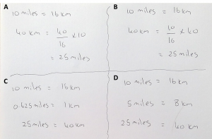
Figure 2: Different methods for solving the conversion rate problem

We could also represent the problem using a ‘ratio table’ (see below). This approach provides a structured layout for working with the relationship between the given miles and kilometre values to find an unknown value.

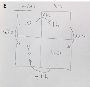
Figure 3: A ratio table method for solving the conversion rate problem

Although each method is equally valid and effective in providing a solution, it can be difficult to see how each method is linked and to understand why each method leads to the same outcome. Many students, particularly lower attaining students, may struggle to recognise that these are simply different ways of working with the same relationship of miles to kilometers rather than completely different methods. The difference in each method relates to how we work with this relationship and the ways in which we choose to adapt the original relationship to work out an unknown value. Also notice that while these methods are effective for finding an answer, they don’t reveal much about the nature of the relationship between miles and kilometers. The method that uses the multiplication ‘×1.6’ in the ratio table is the first method to give direct insight into how miles and kilometers are related proportionally.

Another potential challenge is that none of the methods bear a close resemblance to the problem scenario of distances on a road. This scenario involves a conversion of units on two measurement systems that have different scales – similar to what you might find on a ruler. As such, to support the progressive formalisation of models approach, one possibility would be to choose a ruler-type representation so that there is a natural transition from the realistic scenario to the model and method used to solve the problem. A bar model immediately springs to mind as a potential representation, but the challenge here is that a bar model is an area model showing the relationship of part(s) to a whole, whereas this scenario involves two linear measurement systems. So, it’s difficult to show this problem effectively on a bar model. Instead, a double number-line (DNL) model proves particularly useful here (and, also for any scenario involving a multiplicative relationship between two values).

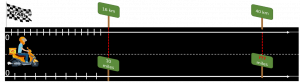
Figure 4: A ‘model of’ the conversion rate problem

Notice in the figure above how the model chosen to represent and explore this problem (the DNL) – the model of this scenario – maps seamlessly to the structure of the problem as represented in the realistic context. This continuity between structure of context and structure is important as it helps students understand why a particular representation has been chosen to model the problem.
To make it easier to work with the model, we can extract the model from the context and present this in a more general form. At any point, however, we could reintroduce or super-impose the context to re-ground and support understanding (for example, if a different or more complex problem is encountered).

Figure 5: A double number line of the conversion rate problem

A DNL is a model comprising two number-lines that have the zero-values aligned but with different scales and variables on each number line. Although DNL’s like the one above are useful because you can count along the line markers to calculate and check answers, they are sometimes difficult and time-consuming to draw because of the difference in scales. As such, more common are ‘empty’ DNL’s such as the one below.

Figure 6: An ‘empty’ double number line of the conversion rate problem

A key benefit of this model is that it provides a single visual resource for:
• exploring and comparing different methods – and, so, for solving the problem (in different ways);
• and, for investigating the nature of the relationship between the variables involved (miles and kilometers in this instance).

This same model can also be used across a range of problems and content topics – which is what makes it an effective model for investigating mathematical structures.

In terms of comparing different methods, consider the double number-line below (the dotted arrow lines indicate a calculation process and the numbers in circles indicate the order of these calculations).

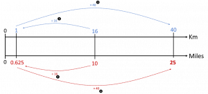
Figure 7: A ‘unit’ method shown on the DNL

This DNL provides a visual map of the different stages involved in the numerical calculation (C) shown above in Figure 2 that involves what is commonly referred to as the ‘unit’ method. In other words, scaling one value down to a single unit, then scaling this value up to the required value, and repeating this series of calculations for the other variable in the relationship. This is also the same method that is used in (B) – which is hard to notice when only looking at the calculations, but easier to spot on the DNL.

Now consider the DNL below.

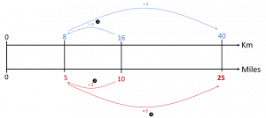
Figure 8: A different scaling method shown on the DNL

This DNL provides a visual map of the steps in the numerical calculation shown in (D) above. This method also involves a scaling approach, but this time halving first and then scaling up by a factor of 5.

By showing both approaches (unit and scaling methods) on the same model, it now becomes easier to have a conversation about how the methods are the same and different, about which method might be more or less efficient, and also about why seemingly different methods both lead to the same result.

Now consider this DNL below.

Figure 9: A third scaling method shown on the DNL

This DNL provides a visual map of the steps in the numerical calculation shown in (A) above and also in the vertical calculation steps in the ratio table in (E) (do you think students easily spot that these are the same calculations?). This method also involves a scaling approach that identifies the direct multiplier from 16 km to 40 km (which is determined by calculating 40 ÷ 16) and applying this same scale factor (of 2.5 in this scenario) to work out the unknown corresponding miles value.

Now consider this final DNL below.

Figure 10: A different method that used the ‘functional relationship’ shown on the DNL

The method used on this DNL is unique and subtly different to all other methods. This is the only method that works directly with the ‘functional’ relationship between the miles and kilometer variables (working ‘between’ the number-lines) to identify that each kilometer value is 1.6 times bigger than its corresponding mile equivalent. This method corresponds to the horizontal calculation on the ratio table in (E). All methods shown on the other DNL’s use a scaling approach that involves scaling within each measurement separately (working ‘along’ the number lines).

A key observation is that the functional relationship defines how these two variables are related – the one variable (kilometres) is 1.6 times larger than the other variable (miles). And, this relationship gives the most efficient way to work with these two variables. So, although working with scalar relationships help us to find the answers to problems involving miles and kilometers, they do not represent the formal relationship between the variables and are commonly not the most efficient way of working.

Now let’s explore what happens if we make a slight adjustment to the DNL by rotating one of the number-lines 90° to the left (slightly beyond the Primary curriculum, but hopefully interesting nonetheless):

[Note that I’ve had to resize the two axes (number-lines) from the original DNL width so that the picture doesn’t take up the whole page!]

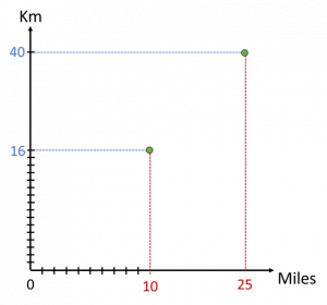
Figure 11: A plot of the conversion rate relationship on a set of axes

We now end up with a set of axes, with each axis containing a different scale and representing a different variable. The ‘functional’ relationship between the two variables (Miles and Km) – the ‘between the lines’ relationship – is represented by dots (●) (or ‘points’) on the space between the axes. Each point represents a relationship between a Miles value and a corresponding Km value such that the Km value is always 1.6 times larger than the Miles value (or the Miles value is 1.6 times smaller than the Km value) – 10 miles and 16 km; 40 km and 25 miles; and so on).

The collection of all of the dots that share this relationship of Km = 1.6 × Miles is a straight line that starts at the origin (0 ; 0) (since 0 Miles is 0 Km – shown on the DNL by both number lines starting at 0):

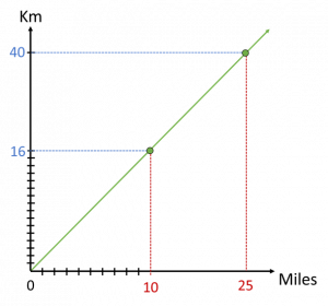
Figure 12: A graphical representation of the conversion rate relationship

Importantly, it is the functional relationship (the relationship between the lines on the DNL) that defines how the variables Miles and Km are related, and it is this relationship that we can represent graphically. Working with the scalar relationships, which commonly represents how many students operate on this type of relationship, does not always give deep insight into the actual nature of the relationship between different variables. This might explain why some students find graph work so difficult and also why some struggle to see the connection between numerical methods and graphical representations of these.

‘Be deliberate, be explicit’
The discussion above has illustrated how a carefully and deliberately chosen representation that bears close resemblance to a contextual situation can be used to both solve a mathematical problem (a model for) and to describe and investigate ways of working with a mathematical relationship (a model of). Although we commonly use representations to help us to understand and then solve problems, less common is the use of these same representations to actively investigate relationships and to explore, compare, contrast and link different methods and ways of working with that relationships.

By being deliberate with the representations that we use and by actively using those representations as models for solving problems and as models of a relationships, we can help students to see the connectedness of different methods and also the connectedness of different representations (for example, the DNL and a line-graph). And, by being explicit about the decisions that we make, we help our students to decode our though process. In keeping with the metacognition tradition, as seen in this EEF guidance report, this supports students’ independent learning behaviours and enables them to reconstruct appropriate problem-solving strategies independently.

In short, the tools that we use are most effective if the are the right tools for the job, if they are used appropriately, and if we communicate clearly to others how to use them.

• Share on Facebook
• Share on Twitter
• Share on Google+
• Share on LinkedIn